Air Propulsion Simulation

Simulating the performance of an air propulsion system as an alternative to solid rocket motors.

For my team was tasked with designing a system capable of moving mining equipment and materials around the surface of the Moon using a propolsive landing. The system had to be tested on earth with something that was feasible for our team to build in 2 semesters. One of the first considerations my capstone advisor wanted was to test the feasibility of an air propulsion system instead of the obvious solution that of using solid rocket motors. This document is really just napkin math to determine if the system is even feasibly and is not mean’t to be a rigorous study of an air propulsion system which would easily keep a capstone team busy by itself.

Show code

using Plots
plotly()
theme(:ggplot2); # In true R spirit

using Unitful
using DataFrames
using Measurements
using Measurements: value, uncertainty
using CSV

The Simulation

An off the shelf paintball gun tank was used for the pressure vessel. This was chosen because they are very high pressure for their weight, and are designed to be bumped around.

# Tank https://www.amazon.com/Empire-Paintball-BASICS-Pressure-Compressed/dp/B07B6M48SR/
V = (85 ± 5)u"inch^3"
P0 = (4200.0 ± 300)u"psi"
Wtank = (2.3 ± 0.2)u"lb"
Pmax = (250 ± 50)u"psi" # Max Pressure that can come out the nozzle

The nozzle diameter was changed until the air prop system had a burn time similar to a G18ST rocket motor.

# Params
d_nozzle = ((1 // 18) ± 0.001)u"inch"
a_nozzle = (pi / 4) * d_nozzle^2

These are just universal values for what a normal day would look like in Arizona. (Çengel and Boles 2015)

# Universal Stuff
P_amb = (1 ± 0.2)u"atm"
γ = 1.4 ± 0.05
R = 287.05u"J/(kg * K)"
T = (300 ± 20)u"K"

The actual simulation is actually quite simple. The basic idea is that using the current pressure you can calculate \(\dot{m}\), which allows calculating the Thrust, and then you can just subtract the current mass of air in the tank by \(\dot{m}\) and recalculate pressure using the new mass then repeat the whole process.

The bulk of the equations in the simulation came from (Çengel and Boles 2015), while the Thrust and \(v_e\) equations came from (Sutton and Biblarz 2001, eq: 2-14).

\[ T = \dot{m} \cdot v_\text{Exit} + A_\text{Nozzle} \cdot (P - P_\text{Ambient}) \]

The initial pressure difference is 4190.0 ± 300.0 psi which is absolutely massive so the area of the nozzle greatly affects the simulation. The paintball tanks do come with pressure regulators, in our case 800 psi which is still a very large number compared to atmospheric pressure. While the total impulse of the system doesn’t really change with different nozzle areas the peak thrust and burn time vary greatly. One of the benefits of doing air propulsion, and the reason it was even considered so seriously, is that it should be possible to vary the nozzle diameter in flight which would make controlled landing much easier.

df = let
t = 0.0u"s"
P = P0 |> u"Pa"
M = V * (P / (R * T)) |> u"kg"
ts = 1u"ms"
df = DataFrame(Thrust=(0 ± 0)u"N", Pressure=P0, Time=0.0u"s", Mass=M)
  while M > 0.005u"kg"
      # Calculate what is leaving tank
      P = minimum([P, Pmax])
      ve = sqrt((2 * γ / (γ - 1)) * R * T * (1 - P_amb / P)^((γ - 1) / γ)) |> u"m/s"
      ρ = P / (R * T) |> u"kg/m^3"
      ṁ = ρ * a_nozzle * ve |> u"kg/s"
  
      Thrust = ṁ * ve + a_nozzle * (P - P_amb) |> u"N"
  
      # Calculate what is still in the tank
      M = M - ṁ * ts |> u"kg"
      P = (M * R * T) / V |> u"Pa"
      t = t + ts
  
      df_step = DataFrame(Thrust=Thrust, Pressure=P, Time=t, Mass=M)
      append!(df, df_step)
  end
  df
end

Analysis

Heres the results plotted. Notice the massive error once the tank starts running low. This is because the calculation for pressure has a lot of variables that are very uncertain. This is mostly due to air being a compressible fluid which is what makes this simulation so difficult to do accurately. The thrust being below 0 N might not make intuitive sense, but its technically possible for the pressure to compress which would leave the inside of the rocket nozzle with a pressure thats actually below atmospheric pressure. The effect would likely last a fraction of a second but the point stands that this simulation is very inaccurate and only meant to get an idea of what an air propulsion system is capable of.

Show code

thrust_values = df.Thrust .|> ustrip .|> value;
thrust_uncertainties = df.Thrust .|> ustrip .|> uncertainty;

air = DataFrame(Thrust=thrust_values, Uncertainty=thrust_uncertainties, Time=df.Time .|> u"s" .|> ustrip);


plot(df.Time .|> ustrip, thrust_values, 
    title="Thrust Over Time", 
    ribbon=(thrust_uncertainties, thrust_uncertainties), 
    fillalpha=.2,label="Thrust",
    xlabel="Time (s)", 
    ylabel="Thrust (N)",
    size = (1200, 800),
    )

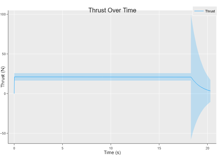
Figure 1: Air Proplsion Simulation

In Figure 2, the air propulsion simulation is compared to commercially available rocket motors. This early in the project we have no idea whether short burns or longer burns are ideal for a propulsive landing so the air propulsion system was compared to a variety of different motors.

Show code

f10 = CSV.read("AeroTech_F10.csv", DataFrame);
f15 = CSV.read("Estes_F15.csv", DataFrame);
g8 = CSV.read("AeroTech_G8ST.csv", DataFrame);


plot(air.Time, air.Thrust, label="Air Propulsion", fillalpha=.1, legend=:topleft, size = (1200, 800));

for (d, l) in [(f10, "F10"), (f15, "F15"), (g8, "G8ST")]
    plot!(d[!,"Time (s)"], d[!, "Thrust (N)"], label=l);
end

title!("Propulsion Comparison");
xlabel!("Time (s)");
ylabel!("Thrust (N)")

Figure 2: Rocket Motor Data: (Coker, n.d.)

Big conclusion about things.