Air Propulsion Simulation

Simulating the performance of an air propulsion system as an alternative to solid rocket motors.

For my team was tasked with designing a system capable of moving mining equipment and materials around the surface of the Moon using a propolsive landing. The system had to be tested on earth with something that was feasible for our team to build in 2 semesters. One of the first considerations my capstone advisor wanted was to test the feasibility of an air propulsion system instead of the obvious solution that of using solid rocket motors. This document is really just napkin math to determine if the system is even feasibly and is not mean’t to be a rigorous study of an air propulsion system which would easily keep a capstone team busy by itself.

Show code

using Plots
plotly()
theme(:ggplot2); # In true R spirit

using Unitful
using DataFrames
using Measurements
using Measurements: value, uncertainty
using CSV

An off the shelf paintball gun tank was used for the pressure vessel. This was chosen because they are very high pressure for their weight, and are designed to be bumped around.

# Tank https://www.amazon.com/Empire-Paintball-BASICS-Pressure-Compressed/dp/B07B6M48SR/
V = (85 ± 5)u"inch^3"
P0 = (4200.0 ± 300)u"psi"
Wtank = (2.3 ± 0.2)u"lb"
Pmax = (250 ± 50)u"psi" # Max Pressure that can come out the nozzle

The nozzle diameter was changed until the air prop system had a burn time similar to a G18ST rocket motor.

# Params
d_nozzle = ((1 // 18) ± 0.001)u"inch"
a_nozzle = (pi / 4) * d_nozzle^2

These are just universal values for what a normal day would look like in Arizona. (Çengel and Boles 2015)

# Universal Stuff
P_amb = (1 ± 0.2)u"atm"
γ = 1.4 ± 0.05
R = 287.05u"J/(kg * K)"
T = (300 ± 20)u"K"

This is the actual simulation. Maybe throw some references in and explain some equations.

The following equations also came from (Çengel and Boles 2015)

The rocket equation is pretty sick(Sutton and Biblarz 2001, eq: 2-14):

\[T = \dot{m} \cdot v_\text{Exit} + A_\text{Nozzle} \cdot (P - P_\text{Ambient}) \] And thats about all you need to get to the Moon(Curtis 2020).

df = let
t = 0.0u"s"
P = P0 |> u"Pa"
M = V * (P / (R * T)) |> u"kg"
ts = 1u"ms"
df = DataFrame(Thrust=(0 ± 0)u"N", Pressure=P0, Time=0.0u"s", Mass=M)
  while M > 0.005u"kg"
      # while t < 30u"s"
      # Calculate what is leaving tank
      P = minimum([P, Pmax])
      ve = sqrt((2 * γ / (γ - 1)) * R * T * (1 - P_amb / P)^((γ - 1) / γ)) |> u"m/s"
      ρ = P / (R * T) |> u"kg/m^3"
      ṁ = ρ * a_nozzle * ve |> u"kg/s"
  
      Thrust = ṁ * ve + a_nozzle * (P - P_amb) |> u"N"
  
      # Calculate what is still in the tank
      M = M - ṁ * ts |> u"kg"
      P = (M * R * T) / V |> u"Pa"
      t = t + ts
  
      df_step = DataFrame(Thrust=Thrust, Pressure=P, Time=t, Mass=M)
      append!(df, df_step)
  end
  df
end

breakdown of the data

"

4 rows × 7 columns

	variable	mean	min	median	max	nmissing	eltype
	Symbol	Quantity	Quantity	Quantity	Quantity	Int64	DataType
1	Thrust	20.0±2.0 N	0.0±0.0 N	21.1±4.7 N	21.1±4.7 N	0	Quantity{Measurement{Float64}, 𝐋 𝐌 𝐓^-2, FreeUnits{(N,), 𝐋 𝐌 𝐓^-2, nothing}}
2	Pressure	2020.0±520.0 psi	40.0±160.0 psi	2010.0±570.0 psi	4200.0±300.0 psi	0	Quantity{Measurement{Float64}, 𝐌 𝐋^-1 𝐓^-2, FreeUnits{(psi,), 𝐌 𝐋^-1 𝐓^-2, nothing}}
3	Time	10.1515 s	0.0 s	10.1515 s	20.303 s	0	Quantity{Float64, 𝐓, FreeUnits{(s,), 𝐓, nothing}}
4	Mass	0.225±0.066 kg	0.005±0.018 kg	0.224±0.071 kg	0.468±0.053 kg	0	Quantity{Measurement{Float64}, 𝐌, FreeUnits{(kg,), 𝐌, nothing}}

"

Heres the results plotted. Notice the massive error once the tank starts running low.

Show code

thrust_values = df.Thrust .|> ustrip .|> value;
thrust_uncertainties = df.Thrust .|> ustrip .|> uncertainty;

air = DataFrame(Thrust=thrust_values, Uncertainty=thrust_uncertainties, Time=df.Time .|> u"s" .|> ustrip);


plot(df.Time .|> ustrip, thrust_values, 
    title="Thrust Over Time", 
    ribbon=(thrust_uncertainties, thrust_uncertainties), 
    fillalpha=.2,label="Thrust",
    xlabel="Time (s)", 
    ylabel="Thrust (N)",
    size = (1200, 800),
    )

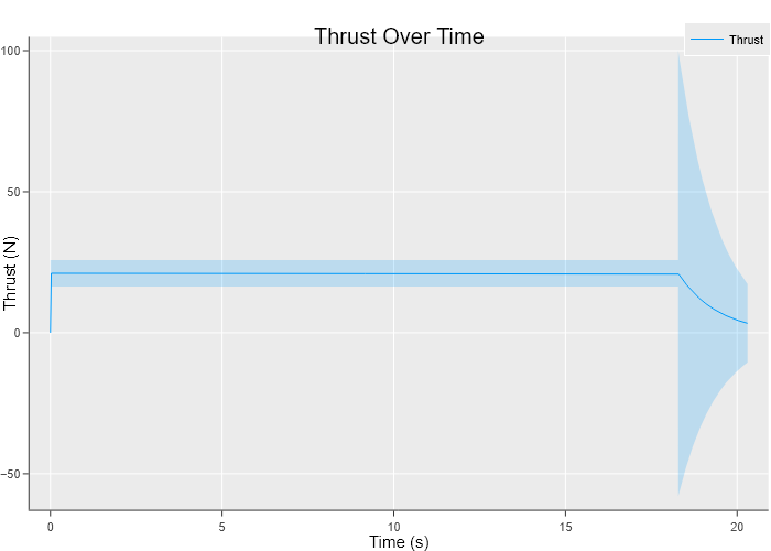
Figure 1: Air Proplsion Simulation

Here the air prop is plotted along with rocket motors that are being

Show code

f10 = CSV.read("AeroTech_F10.csv", DataFrame);
f15 = CSV.read("Estes_F15.csv", DataFrame);
g8 = CSV.read("AeroTech_G8ST.csv", DataFrame);


plot(air.Time, air.Thrust, label="Air Propulsion", fillalpha=.1, legend=:topleft, size = (1200, 800));

for (d, l) in [(f10, "F10"), (f15, "F15"), (g8, "G8ST")]
    plot!(d[!,"Time (s)"], d[!, "Thrust (N)"], label=l);
end

title!("Propulsion Comparison");
xlabel!("Time (s)");
ylabel!("Thrust (N)")

Figure 2: Rocket Motor Data: (Coker, n.d.)

Big conclusion about things.