Report-2

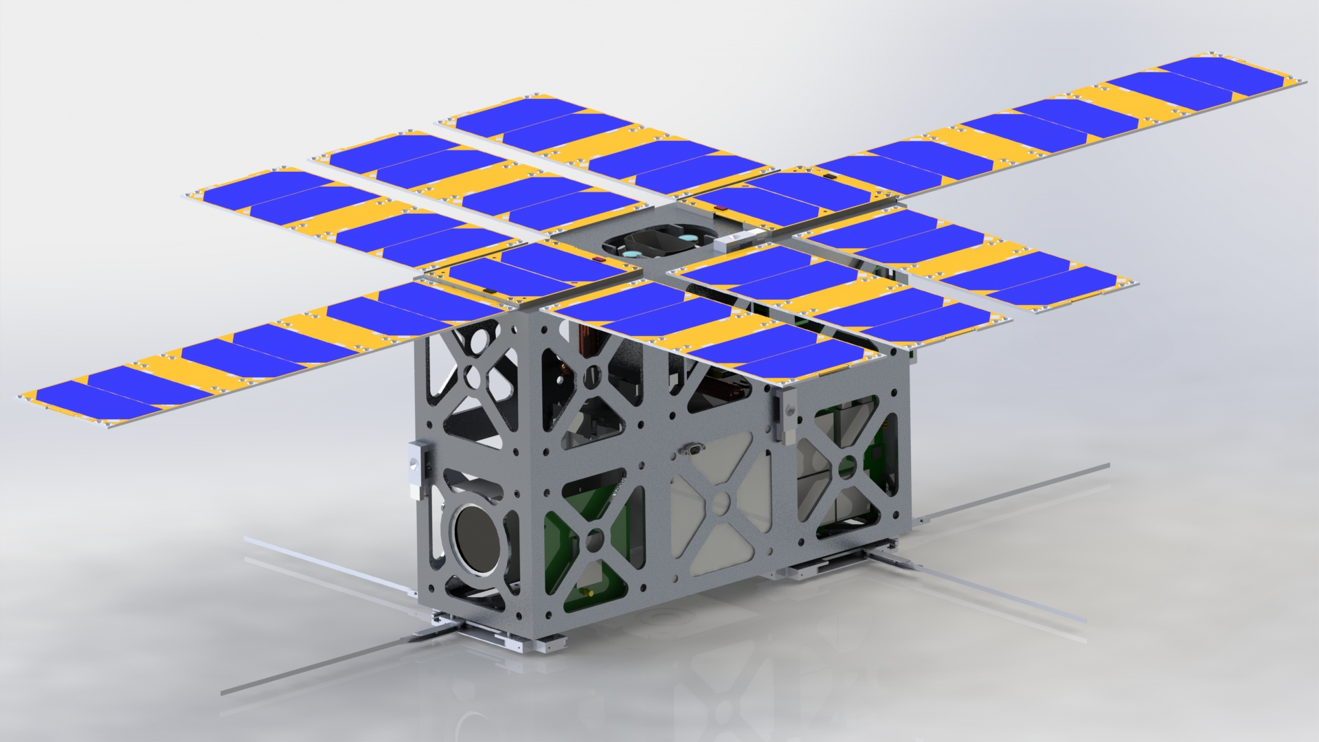
To get started on the project before any scans of the actual debris are made available, I opted to find 3D models online and process them as if they were data collected by my team. GrabCAD is an excellent source of high-quality 3D models, and all of the models have, at worst, a non-commercial license making them suitable for this study. The current dataset uses three separate satellite assemblies found on GrabCAD, below is an example of one of the satellites that was used.

Data Preparation

The models were processed in Blender, which quickly converted the assemblies to stl files, giving 108 unique parts to be processed. Since the expected final size of the dataset is expected to be in the magnitude of the thousands, an algorithm capable of getting the required properties of each part is the only feasible solution. From the analysis performed in Report 1, we know that the essential debris property is the moments of inertia which helped narrow down potential algorithms. Unfortunately, this is one of the more complicated things to calculate from a mesh, but thanks to a paper from [@eberlyPolyhedralMassProperties2002] titled Polyhedral Mass Properties, his algorithm was able to be implemented in the Julia programming language. The current implementation of the algorithm calculates a moment of inertia tensor, volume, and center of gravity in a few milliseconds per part.

The algorithm's speed is critical not only for the eventually large number of debris pieces that have to be processed, but many of the data science algorithms we plan on performing on the compiled data need the data to be normalized. I have decided that it makes the most sense to normalize the dataset based on volume. I chose volume for a few reasons, namely because it was easy to implement an efficient algorithm to calculate volume, and currently, volume seems to be the least essential property for the data analysis. Unfortunately, scaling a model to have a specific volume is an iterative process, but can be done very efficiently using derivative-free numerical root-finding algorithms. The current implementation can scale and process all the properties using only 30% more time than getting the properties without first scaling.

 Row │ variable  mean         min           median       max
     │ Symbol    Float64      Float64       Float64      Float64
─────┼────────────────────────────────────────────────────────────
   1 │ volume     0.00977609   1.05875e-10   2.0558e-5   0.893002
   2 │ cx        -0.836477    -3.13272      -0.00135877  0.0866989
   3 │ cy        -1.52983     -5.07001      -0.101678    0.177574
   4 │ cz         0.162855    -6.83716       0.00115068  7.60925
   5 │ Ix         0.00425039  -5.2943e-7     9.10038e-9  0.445278
   6 │ Iy         0.0108781    1.05468e-17   1.13704e-8  1.14249
   7 │ Iz         0.0111086    1.05596e-17   2.1906e-8   1.15363

Above is a summary of the current 108 part dataset without scaling. The max values are well above the median, and given the dataset's small size, there are still significant outliers in the dataset. For now, any significant outliers will be removed, with more explanation below, but hopefully, this will not become as necessary or shrink the dataset as much as the dataset grows. As mentioned before, a raw and a normalized dataset were prepared, and the data can be found below:

Characterization

The first step toward characterization is to perform a principal component analysis to determine the essential properties. In the past, moments of inertia have been the most important for capturing the variation in the data. However, since this dataset is significantly different from the previous one, it is essential to ensure inertia is still the most important. We begin by using the pca function in Matlab on our scaled dataset.

[coeff,score,latent] = pca(scaled_data);

We can then put the coeff and score returned by the pca function into a biplot to visualize what properties are the most important easily. Unfortunately, we exist in a 3D world, so the centers of gravity and moments of inertia have to be analyzed individually.

The components of all six properties are represented in each of the biplots by the blue lines, and the red dots represent the scores of each property for each part. The data variation is captured pretty well for the current dataset by both the inertia and the center of gravity. I will continue using inertia since it performed slightly better here and was the best when it was performed on just a single satellite. As the dataset grows and the model ingestion pipeline becomes more robust, more time will be spent analyzing the properties.

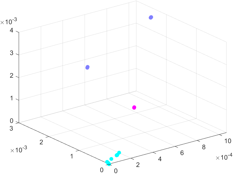
Now that it has been determined that inertia will be used, k-means clustering can be performed on the raw, unscaled dataset.

[IDX, C] = kmeans(inertia,3);

histcounts(IDX) % Get the size of each cluster
    89    10     8

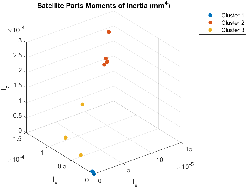
This data has four distinct groups, with much overlap in the larger groups. Therefore, to get a better view, only the smallest magnitude group will be kept since it seems to have the most variation and k-means will be performed again to understand the data better.

inertia = inertia(IDX == 1,:);
[IDX, C] = kmeans(inertia,3);

histcounts(IDX) % Get the size of each cluster
    76     6     7

This brings the dataset down to 89 parts from the original 108 and still leaves some small clusters. This highlights the need to grow the dataset by around 10x so that, hopefully, there will not be so many small, highly localized clusters.

Next Steps

The current dataset needs to be grown in both the amount of data and the variety of data. The most glaring issue with the current dataset is the lack of any debris since the parts are straight from satellite assemblies. Getting accurate properties from the current scans we have is an entire research project in itself, so hopefully, getting pieces that are easier to scan can help bring the project back on track. The other and harder-to-fix issue is finding/deriving more data properties. Properties such as cross-sectional or aerodynamic drag would be very insightful but are likely to be difficult to implement in code and significantly more resource intensive than the current properties the code can derive. Characteristic length is being used heavily by NASA Debrisat and seems straightforward to implement so that will be the next goal for the mesh processing code. Before the next report, I would like to see this dataset grow closer to one thousand pieces.